Markov Chains and Principal Eigenvectors in Network Centrality: PageRank

The pipeline for training a Graph Neural Network can be schematized as follows: Input graph → Structural features → Learning algorithm → Prediction One of the most challenging aspects of this pipeline is the design of structural features. These features aim to capture the essential patterns and relationships within the graph. Automating this process is a key goal in graph machine learning, and it is commonly referred to as feature engineering.

These are few of the possible node level features:

• node degree (treats all neighbours equally)
• node centrality
• clustering coefficient
• graphlets

Different ways to enstablish these features from a graph are:

• engienvector centrality
• betweenness centrality
• closeness centrality (how close to the network)
• and many others

Engienvector centrality

A node $\large v$ is important if surrounded by important neighboring nodes

$$\large c_v=\frac{1}{\lambda}\sum_{u \in N(v)} c_u$$

$\lambda$ is a positive constant, it is used to normalize. The basic notion of this feature engineering task is “The more important my friends the more important I am”.

The last equation can be expressed in a matrix form:

$$\large \lambda \cdot c= A \cdot c \quad (1)$$

This is an eigenvector/eigenvalue equation.

As we will see later, if the graph is undirected and connected, by Perron-Frobenius Theorem the largest eigenvalue is always positive and unique, and the corresponding eigenvector is strictly positive.

The leading eigenvector $\large c_{max}$ is used as a centrality score.

It’s not about how many nodes are connected with you, but how important are the nodes that are connected with you.

Eigenvector centrality measures a node’s importance based on of its neighbors, assigning higher scores to nodes connected to other influential nodes. PageRank extends this idea by introducing a damping factor, which simulates random jumps across the network. This adjustment makes PageRank more robust to dangling nodes (nodes with no outgoing links) and spider traps (subgraphs that can trap random walks), which can distort standard eigenvector centrality. By computing PageRank, one effectively obtains a principal eigenvector of the Google matrix, and the resulting scores can be used as features that capture both the structural connectivity and influence propagation in the network. Compared to pure eigenvector centrality, PageRank provides more stable and meaningful importance values, making it a better choice for feature extraction in graph-based learning tasks.

The web is a directed graph

Link analysis algorithms:

• Pagerank
• Personalized page rank
• Random walk with restarst

The PageRank idea:

• All in-links are not equal: some are more important than others
• Recursive nature, the importance of a node is carried by the importance of other nodes.
• A “vote” from an important page is worth more:

If a page $\large i$ with importance $\large r_i$ has $\large d_i$ out-links, each link gets $\Large \frac{r_i}{d_i}$ votes. Page $\large j$‘s own importance $\large r_j$ is the sum of the votes n its in-links.

So we can define “rank” $\large r_j$ for a node $\large j$ to be:

$$\large r_j = \sum_{i \to j} \frac{r_i}{d_i} \quad (2)$$

$d_i$ … out degree of node $\large i$.

It’s possible to solve this as a system using gaussian elimination, but it’s not scalable.

We can represent the last equation using the matrix form, we have to introduce the Markov matrix or also called stochastic adjacency matrix. More theory about the Markov stochastic matrix later.

Let page $\large j$ have $\large d_j$ out-links. If $\large j \to i$, then $\large M_{ij} = 1/d_j$.

$\large M$ is a column stochastic matrix, this means that every column sums to 1. Now we can write the equation (2) in matrix form as:

$$r = M \cdot r \quad(3)$$

Solving systems of linear equations is a frequent necessity for Web search applications, but the magnitude of computations is usually too large for direct solution methods based on Gaussian elimination to be effective. Consequently, iterative techniques are often the only choice, and, because of size, sparsity, and memory considerations, the preferred algorithms are the simpler methods based on matrix-vector products that require no additional storage beyond that of the original data. Linear stationary iterative methods are the most common.

Appreciate the similarity between this equation and the (1) equation, the only difference is that $\large A$ is the adjacency matrix, while $\large M$ is the Markov matrix or stochastic matrix.

Connection to random walk:

Imagine a random surfer that at some time $\large t$ is on some page $\large i$. at time $\large t+1$ te surfer follow an out-link from $\large i$ uniformly at random.

Eventually it ends up in a page $\large j$ linked from $\large i$.

let $\large p(t)$ be the vector whose $\large i^{th}$ coordinates is the probability that the surfer is at page $\large i$ at time $\large t$. So $\large p(t)$ is a probability distribution over pages.

To compute where the surfer will be at the time $\large t+1$ we can apply it to the left the column stochastic matrix.

$$\large p(t+1) = M \cdot p(t) \quad (4)$$

The entry $\large p_j(t+1)$ gives the probability that the surfer is on node $\large j$ at time $\large t+1$. It is computed by summing the contributions from all nodes that link to $\large j$. Formally:

$$\large p_j(t+1) = \sum_{i \to j} M_{ij} \, p_i(t)$$

Suppose the random walk reaches a state where:

$$p(t+1) = M \cdot p(t) = p(t)$$

Then $\large p(t)$ is stationary distribution of random walk. Our original rank vector $\large r$ satisfies $\large r = M \cdot r$, that means that our vector $\large r$ is a stationary distribution for the random walk!

How do we solve the equation:

$$\large 1\cdot r = M r$$

Starting from any vector $u$, the limit $M(M(... M(Mu)))$ is the long-term distribution of the surfers. When applying a linear map $u \to Mu$ again and again, we obtain a discrete dynamical system. We want to understand what happens with the orbit $u_{1} = M u, u_{2} = MMu , u_{3}=MMMu$, … and find a closed formula for $M^n u$.

For example:

The one-dimensional discrete dynamical system $x \to ax$ or $x_{n+1} = ax_n$ has the solution $x_n = a^nx_{0}$. The value $1.0320 · 1000 = 1806.11$ for example is the balance on a bank account which had $1000$ dollars 20 years ago if the interest rate was a constant $3$ percent.

If $u$ is an eigenvector with eigenvalue $\lambda$, then $Mu = λu, M^2u = M(Mu)) = Mλu = λMu = λ^2u$ and more generally $M^n u = λ^n u$.

Summary:

• PageRank measures importance of nodes in a graph using the link structure of the web
• Yo can simulate a random web surfer using stochastic adjacency matrix M
• PageRank solves $\large r = M \cdot r$ where $\large r$ can be viewed as both the principle eigenvector of $\large M$ and as the stationary distribution of a random walk over the graph.

Important questions

At this point we have an intuitive knowledge of how this algorithm works, but to properly understand the essence of it, it’s necessary to dive into the mathematics that lies behind the algorithm. We ought to ask ourself these important questions:

• Will this iterative process continue indefinitely or will it converge?
• Under what circumstances or properties of H is it guaranteed to converge?
• Will it converge to something that makes sense in the context of the PageRank problem?
• Will it converge to just one vector or multiple vectors?
• Does the convergence depend on the starting vector π(0)T ?
• If it will converge eventually, how long is “eventually”? That is, how many iterations can we expect until convergence? In the following part of the article, I’m going to answer this questions and provide and example of this algorithm give an instance.

---

Power iteration

Iterative procedure that will update over time our rank vector $\large r$. We start initiating every node with an initial state, continue the process until the states stabilizes.

Repeat until convergence:

$$r_j^{t+1}=\sum_{i \to j} \frac{r_j^t}{d_i}$$

Initialize $\large r^0 = [\frac{1}{N}, \dots, \frac{1}{N}]^T$ Iterate: $\large r^{t+1} = M r^t$ that is the same of $\large r_j^{t+1}=\sum_{i \to j} \frac{r_j^t}{d_i}$ Stop when $\large |r^{t+1}-r^t| < \epsilon$

About 50 iterations is sufficient to estimate the limiting solution.

---

Markov matrix

A discrete-time Markov chain is a sequence of random variables $X_1, X_2, X_3, \ldots$ with the Markov property, namely that the probability of moving to the next state depends only on the present state and not on the previous states:

$$\Pr\!\left( X_{n+1} = x \;\middle|\; X_1 = x_1, X_2 = x_2, \ldots, X_n = x_n \right) = \Pr\!\left( X_{n+1} = x \;\middle|\; X_n = x_n \right),$$

If both conditional probabilities are well defined, that is, if

$$\Pr\!\left( X_1 = x_1, \ldots, X_n = x_n \right) > 0.$$

The possible values of $X_i$ form a countable set $S$ called the state space of the chain.

The matrix describing the markov chain is called transition matrix, but it’s also very common to call it stochastic matrix.

A stochastic matrix is an $\large n \times n$ matrix where all entries are nonnegative and each row adds up to 1.

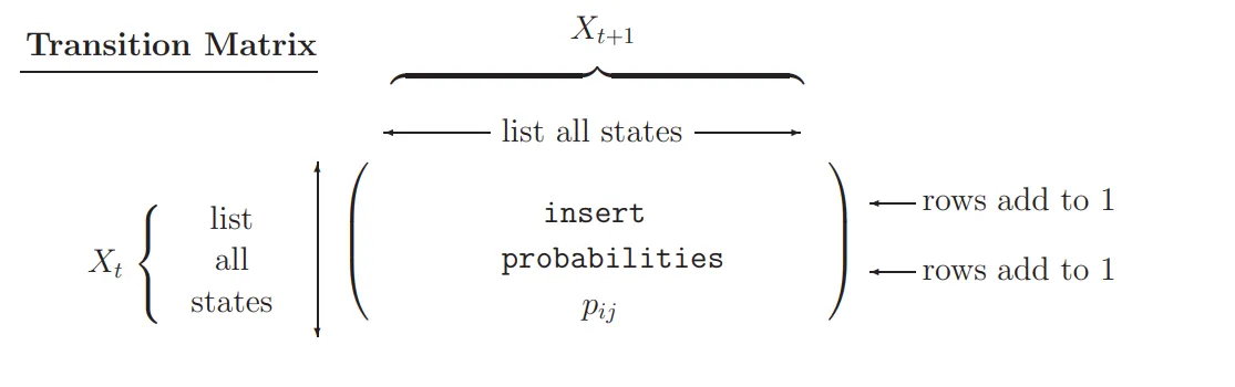
• The ROWS represent NOW, or FROM $(X_t)$;
• The COLUMNS represent NEXT, or TO $(X_t+1)$;
• Entry $(i, j)$ is the CONDITIONAL probability that $NEXT = j$, given that $NOW = i$: the probability of going FROM state $i$ TO state $j$.

$$p_{ij} = \mathbb{P}(X_{t+1} = j | X_t=i)$$

A probability vector or stochastic vector is a vector with non-negative entries that add up to one.

Proof:

Consider the transpose matrix $A^T$. Since $A$ is row-stochastic, the sum of the entries in each row of $A$ is $1$, which means that the sum of the entries in each column of $A^T$ is $1$. Thus

$$A^T \begin{bmatrix} 1 \\ 1 \\ \vdots \\ 1 \end{bmatrix} = \begin{bmatrix} 1 \\ 1 \\ \vdots \\ 1 \end{bmatrix},$$

so $A^T$ has eigenvalue $1$ with eigenvector $\mathbf{1} = (1,1,\ldots,1)^T$.
Since $A$ and $A^T$ have the same characteristic polynomial, they share the same eigenvalues. Therefore, $A$ also has eigenvalue $1$.

Now suppose $v$ is an eigenvector of $A$ with eigenvalue $\lambda$ such that $|\lambda| > 1$. Then

$$A^n v = \lambda^n v,$$

which grows in length exponentially as $n \to \infty$. In particular, for large $n$, some entry of $A^n v$ must have magnitude larger than $1$.

However, $A^n$ is also row-stochastic (this can be shown by induction), so all its entries are nonnegative and each row sums to $1$. Hence every entry of $A^n$ is bounded by $1$, and multiplying $A^n$ by any probability vector produces another probability vector. This contradicts the assumption that an eigenvalue with $|\lambda| > 1$ exists.

Therefore, all eigenvalues $\lambda$ of $A$ satisfy $|\lambda| \leq 1$, with $1$ always being an eigenvalue.

---

Perron–Frobenius Theory

In a presentation held by Hans Schneider titled “Why I Love Perron–Frobenius”, he addressed how the Perron-Frobenius theory of nonnegative matrices is not only extremely useful, but it is also among the most beautiful theories in mathematics.

The applications involving PageRank, HITS, and other ranking schemes help to underscore this principle. A matrix A is said to be nonnegative when each entry is a nonnegative number (denote this by writing $\large A ≥ 0$). Similarly, $\large A$ is a positive matrix when each $\large a_{ij}$ > 0 (write $\large A > 0$). For example, the hyperlink matrix H and the stochastic matrix M that are at the foundation of PageRank are nonnegative matrices, and the Google matrix G is a positive matrix. Consequently, properties of positive and nonnegative matrices govern the behavior of PageRank, and the Perron–Frobenius theory reveals these properties by describing the nature of the dominant eigenvalues and eigenvectors of positive and nonnegative matrices.

For a matrix $A$, the spectral radius is defined as

$$\rho(A) = \max \{ |\lambda| : \lambda \in \sigma(A) \},$$

that is, the maximum absolute value among the eigenvalues of $A$.

In Perron’s theorem, we set $r = \rho(A)$, meaning that the eigenvalue under consideration is precisely the one with the largest modulus.
For positive matrices ($A > 0$), this eigenvalue $r$ is real, positive, simple, and associated with an eigenvector having all positive components.

Perron’s theorem for positive matrices is a powerful result, so it’s only natural to ask what happens when zero entries appear. Not all is lost if we are willing to be flexible. The next theorem says that part of Perron’s theorem for positive matrices can be extended to nonnegative matrices by sacrificing the existence of a positive eigenvector for a nonnegative one.

Perron’s Theorem for Nonnegative Matrices

Irreducibility and Connectivity

Perron-Frobenius Theorem

Frobenius’s contribution was to realize that while properties 1, 3, 4, and 6 in Perron’s theorem for positive matrices can be lost when zeros creep into the picture (i.e., for nonnegative matrices), the trouble is not simply the existence of zero entries, but rather the problem is the location of the zero entries. In other words, Frobenius realized that the lost properties 1, 3, and 4 are in fact not lost when the zeros are in just the right locations—namely the locations that ensure that the matrix is irreducible. Unfortunately irreducibility alone still does not save property 6— it remains lost.

Irreducible Markov Chains

Analyzing limiting properties of Markov chains requires that the class of stochastic matrices (and hence the class of stationary Markov chains) be divided into four mutually exclusive categories.

1. M is irreducible with $\displaystyle \lim_{k \to \infty} M^k$ existing
   (i.e., M is primitive).

2. M is irreducible with $\displaystyle \lim_{k \to \infty} M^k$ not existing
   (i.e., M is imprimitive).

3. M is reducible with $\displaystyle \lim_{k \to \infty} M^k$ existing.

4. M is reducible with $\displaystyle \lim_{k \to \infty} M^k$ not existing.

Let $\large P$ be the transition probability matrix for an irreducible Markov chain on states $\{S_1, S_2, \dots, S_n\}$, and let $\large \pi^T$ be the left-hand Perron vector for $\large P$ (i.e., $\large \pi^T P = \pi^T$, $\|\pi\|_1 = 1$).

The following hold for every initial distribution $p^T(0)$:

• The $k^{th}$ step transition matrix is $P^k$.
  The $\large (i,j)$-entry in $P^k$ is the probability of moving from $S_i$ to $S_j$ in exactly $k$ steps.

• The $k$th step distribution vector is given by

  $$p^T(k) = p^T(0) P^k$$

• If $P$ is primitive (aperiodic), and if $\large e$ is the column vector of all 1’s, then

  $$\lim_{k \to \infty} P^k = e \pi^T \quad \text{and} \quad \lim_{k \to \infty} p^T(k) = \pi^T$$

• If $P$ is imprimitive (periodic), then

  $$\lim_{k \to \infty} \frac{I + P + \cdots + P^{k-1}}{k} = e \pi^T$$

  and

  $$\lim_{k \to \infty} \frac{p^T(0) + p^T(1) + \cdots + p^T(k-1)}{k} = \pi^T$$

• Regardless of whether $P$ is primitive or imprimitive, the $j^{th}$ component $\pi_j$ of $\pi^T$ represents the long-run fraction of time that the chain is in $S_j$.

• The vector $\pi^T$ is the unique stationary distribution vector for the chain, because it is the unique probability distribution satisfying

  $$\large \pi^T P = \pi^T$$

So we have seen that a unique positive PageRank vector exists when the Google matrix is stochastic and irreducible. Further, with the additional property of aperiodicity, the power method will converge to this PageRank vector, regardless of the starting vector for the iterative process.

Implementation

Problems to handle: If there are:

• pages with dead ends (have no out-links)
• Spider traps (all out-links are within the group) Our random walk could fail. The solution for spider traps is teleport, at each time step, the random surfer has two options:
• with probability $\beta$, follows a link at random
• with probability $1-\beta$, jump to a random page
• Common value for $\beta$ are 0.8 to 0.9

For dead ends, the solution is teleport with probability $\large 1$. The spider traps are not a mathematical problem, simply the result is not what we want. On the contrary, Dead-ends are a mathematical problems since our matrix wouldn’t be anymore a column stochastic matrix.

This allows us to the final matrix, also called the google matrix, it has the shape of:

$$G_{ij} = \begin{cases} \beta \dfrac{A_{ij}}{\sum\limits_{i} A_{ij}} + (1-\beta)\dfrac{1}{N}, & \text{if } \sum\limits_{i} A_{ij} \neq 0, \\[1.2em] \dfrac{1}{N}, & \text{otherwise.} \end{cases} \quad \text{with } \beta = 0.85$$

Where in this case $\large \dfrac{A_{ij}}{\sum\limits_{i} A_{ij}}$ is just the stochastic matrix $\large M$. Here we don’t simulate the random walk, we think of it of being run infinitely long, computing this is equal to solve this recurvie equation by computing the leading eigevector of G.

So random walk is just an intuition that we never truly simulate.

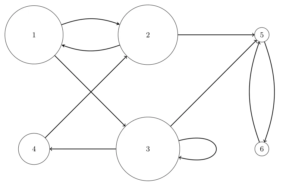
Example:

Take this graph, the goal will be to extract the feature that better represent the importance of each node in the over all graph.

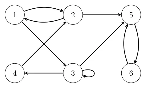
The first step through the process is to represent the graph as an adjacency matrix:

The matrix is going to be a $\large 6 \times 6$ matrix. We set $\large A_{i,j} = 1$ if page $\large j$ has a link to page $\large i$ and $\large A_{i,j} = 0$ otherwise.

$$\large A = \begin{bmatrix} 0 & 1 & 1 & 0 & 0 & 0 \\[4pt] 1 & 0 & 0 & 0 & 1 & 0 \\[4pt] 0 & 0 & 1 & 1 & 1 & 0 \\[4pt] 0 & 1 & 0 & 0 & 0 & 0 \\[4pt] 0 & 0 & 0 & 0 & 0 & 1 \\[4pt] 0 & 0 & 0 & 0 & 1 & 0 \end{bmatrix}$$

Note that the $\large 1$ in the diagonal happen only if there is a self loop.

Next we are going to assume that every link in that column are equally likely (equal probability out-links), so we divide every single entry of a column by the number of $\large 1$ in that column. Since the columns must summ up to 1.

$$\large M = \begin{bmatrix} 0 & 1/2 & 1/2 & 0 & 0 & 0 \\[4pt] 1 & 0 & 0 & 0 & 1/3 & 0 \\[4pt] 0 & 0 & 1/2 & 1 & 1/3 & 0 \\[4pt] 0 & 1/2 & 0 & 0 & 0 & 0 \\[4pt] 0 & 0 & 0 & 0 & 0 & 1 \\[4pt] 0 & 0 & 0 & 0 & 1/3 & 0 \end{bmatrix}$$

Now we need to eliminate spider-traps and dead-ends.

Do have this result we have to use the definition of google matrix I provided before:

$$G_{ij} = \begin{cases} \beta \dfrac{A_{ij}}{\sum\limits_{i} A_{ij}} + (1-\beta)\dfrac{1}{N}, & \text{if } \sum\limits_{i} A_{ij} \neq 0, \\[1.2em] \dfrac{1}{N}, & \text{otherwise.} \end{cases} \quad \text{with } \beta = 0.85$$ $$\large G = 0.85 \cdot \begin{bmatrix} 0 & 1/2 & 1/2 & 0 & 0 & 0 \\[4pt] 1 & 0 & 0 & 0 & 1/3 & 0 \\[4pt] 0 & 0 & 1/2 & 1 & 1/3 & 0 \\[4pt] 0 & 1/2 & 0 & 0 & 0 & 0 \\[4pt] 0 & 0 & 0 & 0 & 0 & 1 \\[4pt] 0 & 0 & 0 & 0 & 1/3 & 0 \end{bmatrix} + 0.15 \cdot \begin{bmatrix} 1/6 & 1/6 & 1/6 & 1/6 & 1/6 & 1/6 \\[4pt] 1/6 & 1/6 & 1/6 & 1/6 & 1/6 & 1/6 \\[4pt] 1/6 & 1/6 & 1/6 & 1/6 & 1/6 & 1/6 \\[4pt] 1/6 & 1/6 & 1/6 & 1/6 & 1/6 & 1/6 \\[4pt] 1/6 & 1/6 & 1/6 & 1/6 & 1/6 & 1/6 \\[4pt] 1/6 & 1/6 & 1/6 & 1/6 & 1/6 & 1/6 \end{bmatrix}$$

The middle step for computing this summation of matrixes is this:

$$G = \begin{bmatrix} 0 & 17/40 & 17/40 & 0 & 0 & 0 \\[4pt] 17/20 & 0 & 0 & 0 & 17/60 & 0 \\[4pt] 0 & 0 & 17/40 & 17/20 & 17/60 & 0 \\[4pt] 0 & 17/40 & 0 & 0 & 0 & 0 \\[4pt] 0 & 0 & 0 & 0 & 0 & 17/20 \\[4pt] 0 & 0 & 0 & 0 & 17/60 & 0 \end{bmatrix} + \begin{bmatrix} 1/40 & 1/40 & 1/40 & 1/40 & 1/40 & 1/40 \\[4pt] 1/40 & 1/40 & 1/40 & 1/40 & 1/40 & 1/40 \\[4pt] 1/40 & 1/40 & 1/40 & 1/40 & 1/40 & 1/40 \\[4pt] 1/40 & 1/40 & 1/40 & 1/40 & 1/40 & 1/40 \\[4pt] 1/40 & 1/40 & 1/40 & 1/40 & 1/40 & 1/40 \\[4pt] 1/40 & 1/40 & 1/40 & 1/40 & 1/40 & 1/40 \\[4pt] \end{bmatrix}$$

As the final result, you can see how the property of stochastic matrix remained, but we have a full matrix that avoid problems like spider-traps and dead-ends.

$$G = \begin{bmatrix} 1/40 & 18/40 & 18/40 & 1/40 & 1/40 & 1/40 \\[4pt] 35/40 & 1/40 & 1/40 & 1/40 & 37/120 & 1/40 \\[4pt] 1/40 & 1/40 & 18/40 & 35/40 & 37/120 & 1/40 \\[4pt] 1/40 & 18/40 & 1/40 & 1/40 & 1/40 & 1/40 \\[4pt] 1/40 & 1/40 & 1/40 & 1/40 & 1/40 & 35/40 \\[4pt] 1/40 & 1/40 & 1/40 & 1/40 & 37/120 & 1/40 \\[4pt] \end{bmatrix}$$

Now we can iterate until we find a stable state:

• Initialize $\large r^0 = [\frac{1}{N}, \dots, \frac{1}{N}]^T$
• Iterate: $\large r^{t+1} = M \cdot r^t$
• Stop when $\large \lvert r^{t+1} - r^t \rvert < \epsilon$

After few iteration (according to the epsilon you chose), you will arrive in a stable solution that in my case is:

$$\large r = \begin{bmatrix} 0.24534 \\ 0.25136 \\ 0.26819 \\ 0.13147 \\ 0.06128 \\ 0.04236 \end{bmatrix} \; \begin{array}{l} \text{Node 1} \\ \text{Node 2} \\ \text{Node 3} \\ \text{Node 4} \\ \text{Node 5} \\ \text{Node 6} \end{array}$$

You can try this for yourself just executing the pythong code you will find below.

from fractions import Fraction

G = [
    [Fraction(1,40), Fraction(18,40), Fraction(18,40), Fraction(1,40), Fraction(1,40), Fraction(1,40)],

    [Fraction(35,40), Fraction(1,40), Fraction(1,40), Fraction(1,40), Fraction(37,120), Fraction(1,40)],

    [Fraction(1,40), Fraction(1,40), Fraction(18,40), Fraction(35,40), Fraction(37,120), Fraction(1,40)],

    [Fraction(1,40), Fraction(18,40), Fraction(1,40), Fraction(1,40), Fraction(1,40), Fraction(1,40)],

    [Fraction(1,40), Fraction(1,40), Fraction(1,40), Fraction(1,40), Fraction(1,40), Fraction(35,40)],

    [Fraction(1,40), Fraction(1,40), Fraction(1,40), Fraction(1,40), Fraction(37,120), Fraction(1,40)]
]

# Initial rank vector (uniform)

r = [Fraction(1,6) for _ in range(6)]

# Stopping threshold epsilon
epsilon = Fraction(1,1000) 

def multiply_matrix_vector(M, vec):

    """Multiply matrix M by column vector vec (both using Fraction)"""
    result = []

    for row in M:

        s = sum(r*c for r,c in zip(row, vec))

        result.append(s)

    return result


def vector_diff(v1, v2):

    """Max absolute difference between two vectors"""

    return max(abs(a-b) for a,b in zip(v1, v2)) 

# Iterative multiplication until convergence

iteration = 0

while True:

    r_next = multiply_matrix_vector(G, r)

    diff = vector_diff(r, r_next)

    iteration += 1

    print(f"Iteration {iteration}: {r_next}  | diff = {diff}")

    if diff < epsilon:

        break

    r = r_next

r_final = [round(float(x), 5) for x in r_next]

print("\nConverged PageRank:")

for i, val in enumerate(r_final, 1):

    print(f"Node {i}: {val}")

This vector represents the importance of the nodes in the graph. A representative image of the importance of nodes in the graph is provided below.

Although node 5 receives links from nodes 2 and 3, its PageRank is relatively small. This is because PageRank distributes a node’s “importance” proportionally across all of its outgoing links. Node 2 and node 3 each link to multiple nodes, so the portion of their rank that reaches node 5 is only a fraction of their total importance. In other words, PageRank measures the probability that a random surfer lands on a node, taking into account both the importance of linking nodes and how their rank is split among their outgoing links. Therefore, even if a node is linked by important nodes, it may still have a low rank if those nodes distribute their rank widely.

References 📚

Research Papers

• Jure Leskovec et al., Pixie: System for Large-Scale Graph Mining, PDF
• Bindel, Lecture Notes CS6210, Cornell University, PDF
• Vesak, Stochastic Processes Notes, PDF

Books

• Horn, R.A. & Johnson, C.R., Matrix Analysis, 2nd Edition, PDF, p. 549
• Langville & Meyer, Google’s PageRank and Beyond, PDF, p. 186
• Horn & Johnson, Matrix Analysis, Chapter 8, PDF

Markov Chains & Linear Algebra

• Knill, Lecture Notes on Markov Chains, Harvard University, Lecture 33, Lecture 34
• Knill, Linear Algebra Probability Summary, Lecture 36
• MathOverflow, Examples on Non-Diagonalizable Stochastic Matrices, Link

Exercises

• Knight, Markov Chains Exercise Sheet with Solutions, PDF
• Probability Course, Solved Problems, Link
• Gordon, Solved Problems on Markov Chains, PDF

Reference Notes

• Fewster, Transition Matrix Definitions, PDF
• Stanford EE363, Perron-Frobenius Theory, PDF
• YouTube, Perron-Frobenius Theory Lecture, Watch